Measuring how much it moves

The Risk and Psychology course spoke of risk in words: how much you can lose, how much a position swings. This chapter gives risk a number. Volatility is the standard deviation of returns, a measure of how much a price bounces around its average day to day, and it is the most common quantitative face of risk. A calm, steady stock has low volatility; a wild one has high volatility, and the same market move means very different things for each. Computing it is two lines.

Volatility in two lines

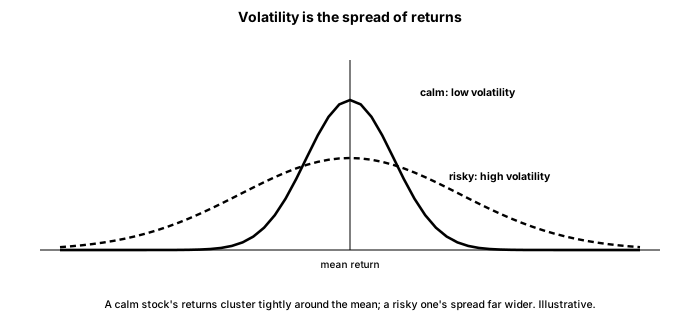
You already have daily returns; volatility is just their standard deviation, with one convention for making it comparable across instruments.

# Volatility is the standard deviation of returns, the quantitative face of risk.
import pandas as pd
import numpy as np

df = pd.read_csv("sample_prices.csv", parse_dates=["Date"], index_col="Date")

returns = df["Close"].pct_change().dropna()
daily_vol = returns.std()
annual_vol = daily_vol * np.sqrt(252)     # about 252 trading days in a year

print(f"Daily volatility:      {daily_vol * 100:.2f}%")
print(f"Annualised volatility: {annual_vol * 100:.2f}%")

Daily volatility:      1.14%
Annualised volatility: 18.14%

The first figure, the standard deviation of the daily returns, is the daily volatility, about 1.14% for this sample, meaning a typical day moves a little over one percent away from the average. On its own that number is hard to compare, so it is conventional to annualise it by multiplying by the square root of the number of trading days in a year, about 252, giving an annualised volatility of roughly 18.14%. Annualised volatility is the figure you usually see quoted, and it lets you compare a placid large-cap against a jumpy small-cap on one scale.

Why the square root, and why it matters

The square root looks odd, so it is worth a word. Volatility grows with the square root of time, not with time itself, because returns partly cancel out over longer periods rather than simply adding, so to scale a daily figure up to a year you multiply by the square root of 252, not by 252. You do not need the proof, but you should know that this is an assumption, and a rough one: it treats each day as independent and identically behaved, which real markets only approximately are. Annualised volatility is a useful, standard estimate, not an exact truth.

The reason this matters for a trader circles back to the earlier course. Volatility is the number behind position sizing: a more volatile instrument needs a smaller position for the same rupee risk, because it moves further against you on an ordinary day. It is the number behind risk-adjusted comparison: a return earned with half the volatility is a better return. And it is the number behind the honest expectations that course insisted on, since high volatility means large drawdowns are normal, not exceptional. Putting a number on how much a price moves is the first step to managing what that movement can do to you.

What to carry forward

Volatility puts a number on how much a price swings: the standard deviation of returns, about 1.14% daily here, annualised to roughly 18% by the square-root-of-252 convention, which is a standard estimate rather than an exact law. It is the quantitative face of the risk from the earlier course, underlying position sizing, risk-adjusted comparison, and honest expectations about drawdowns.

You have now computed returns, trends, and volatility, but numbers in a table are hard to feel. The next chapter draws them, turning the price and its moving averages into a chart you can actually see.