The trader's spreadsheet in code

If NumPy is the engine, pandas is the car you actually drive. It is the single most important tool in this course, because it gives you data structures shaped exactly like market data: labelled columns and labelled tables, indexed by date, with a huge kit of operations for slicing, filtering, and computing. If you have ever used a spreadsheet, pandas will feel familiar, except that here the spreadsheet is programmable, repeatable, and able to handle far more data than a spreadsheet ever could.

The Series and the DataFrame

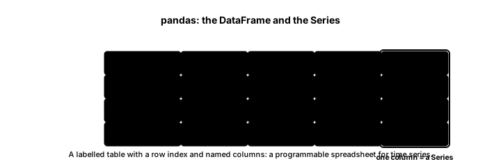
pandas has two core structures. A Series is a single column of values with labels attached, and a DataFrame is a table of such columns sharing one set of row labels, called the index. This program builds one of each.

# pandas gives labelled data: a Series (one column) and a DataFrame (a table).
import pandas as pd

closes = pd.Series([1380, 1402, 1395, 1410, 1425],
                   index=["Mon", "Tue", "Wed", "Thu", "Fri"])
print("Wednesday:", closes["Wed"])     # access by label
print("Mean:", closes.mean())

df = pd.DataFrame(
    {"close": [1380, 1402, 1395, 1410, 1425],
     "volume": [120, 150, 90, 200, 170]},
    index=["Mon", "Tue", "Wed", "Thu", "Fri"],
)
print(df)
print("Average close:", df["close"].mean())

Wednesday: 1395
Mean: 1402.4
     close  volume
Mon   1380     120
Tue   1402     150
Wed   1395      90
Thu   1410     200
Fri   1425     170
Average close: 1402.4

The Series holds five closing prices labelled by weekday, so you can ask for a value by its label, closes["Wed"], and get 1395, rather than remembering it is at position 2. Calling closes.mean() averages the whole Series to 1402.4. The DataFrame is a table with two columns, close and volume, sharing the weekday index, and printing it shows exactly the tidy grid you would expect. Selecting a column by name, df["close"], gives you back a Series, on which .mean() again returns 1402.4. Labels everywhere, and operations that apply to whole columns at once: that is pandas.

Why pandas suits market data

Market data is a labelled table indexed by time, which is precisely what a DataFrame is. Each row is a date; each column is a quantity, open, high, low, close, volume; and almost everything you want to do, compute a return column, filter to volatile days, average by month, is a natural operation on that table. Because pandas is built on NumPy, those operations are vectorised and fast, applying to entire columns at once in the way the last chapter practised, so you rarely write a loop. And because everything is labelled, your code says what it means: df["close"].mean() reads as its intent, where a bare array index would not.

You access data in a DataFrame in two ways that are worth keeping straight: by label, using the row and column names, and by position, using numbers. pandas gives you tools for both, and mixing them up is a common early confusion, so as you practise, notice whether you are asking for something by its name or by its place. Everything else in this part, loading files, cleaning, filtering, and handling dates, is done through the DataFrame, so time spent comfortable with it now pays off in every chapter that follows.

What to carry forward

pandas is the heart of the course: the Series is a labelled column, the DataFrame a labelled table indexed by rows, and together they are a programmable spreadsheet shaped exactly like market data. You access data by label or by position, operate on whole columns at once, and rely on its NumPy-backed speed. Everything ahead, loading, cleaning, filtering, and dates, runs through the DataFrame.

You have been building small tables by hand. Real analysis starts from data you load, and most market data arrives as a file. The next chapter reads a CSV of prices into a DataFrame.