Reading a file of prices

Real analysis starts from real data, and the most common way data reaches you is as a CSV file, a plain text table of comma-separated values, which is what almost every source of historical prices will hand you. pandas reads a CSV into a DataFrame in a single line, and from that moment you have the labelled table from the last chapter, filled with genuine prices, ready to work on. This is the doorway through which most of your data will enter.

One line to load

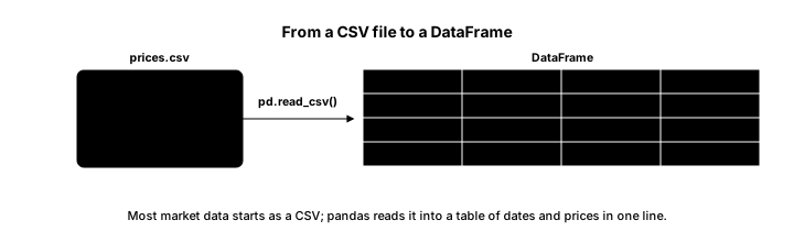
The function is read_csv, and with a couple of sensible options it does exactly what you want. This program loads a saved file of daily prices.

# Read a file of prices into a pandas DataFrame.
import pandas as pd

df = pd.read_csv("sample_prices.csv", parse_dates=["Date"], index_col="Date")

print("Shape (rows, columns):", df.shape)
print(df.head())
print("Columns:", list(df.columns))

Shape (rows, columns): (180, 5)
               Open     High      Low    Close  Volume
Date                                                  
2024-01-01  1406.26  1411.83  1401.56  1408.90   52573
2024-01-02  1410.76  1419.41  1400.77  1407.13   85367
2024-01-03  1423.20  1423.82  1415.62  1418.63  287804
2024-01-04  1443.04  1447.45  1434.72  1445.13  411752
2024-01-05  1442.61  1446.59  1427.39  1441.64  372918
Columns: ['Open', 'High', 'Low', 'Close', 'Volume']

The load is one line, and the two options earn their place. parse_dates=["Date"] tells pandas to treat the Date column as real dates rather than plain text, and index_col="Date" makes that date column the index of the table, so each row is labelled by its date. The output confirms the result: a shape of 180 rows and 5 columns, a head showing the first five days with their open, high, low, close, and volume, each row stamped with its date, and a list of the columns. In one line you have gone from a file on disk to a clean, date-indexed table.

(The file here is a saved sample so the course runs without a live data connection. The next chapter shows how to fetch real prices, which arrive in exactly this shape.)

Inspect, and save

Two habits go with loading. First, always look at what you loaded before trusting it, which the next chapter covers in full, but even here df.shape and df.head() are the first glance: do the dimensions look right, are the columns the ones you expected, do the first few rows look sane. A surprising number of analysis errors are really loading errors, a wrong separator, a header read as data, a column of numbers loaded as text, and a quick look catches them early.

Second, just as read_csv reads a file in, df.to_csv("filename.csv") writes a DataFrame back out, which you use to save a cleaned dataset or the results of an analysis so you need not recompute them next time. Reading and writing CSVs is the everyday plumbing of data work, and pandas makes both a single call.

What to carry forward

A CSV is the usual doorway for market data, and pandas read_csv loads it into a date-indexed DataFrame in one line, with parse_dates and index_col doing the useful setup. Glance at shape and head immediately to catch loading errors, and use to_csv to save your work. This is the everyday plumbing you will use constantly.

Files are one source of data, but you often want prices on demand rather than from a saved file. The next chapter fetches real market data programmatically, through a broker's SDK or an open library.