Managing the whole book's risk

A quant manages risk at the level of the whole portfolio, not the single trade, and with more tools than the earlier risk course had room for. This chapter covers measuring portfolio risk, including the value-at-risk measure Risk and Psychology deferred to here, controlling exposure to each factor, and the discipline of turning a strategy off when it breaks.

Value-at-Risk, and its blind spot

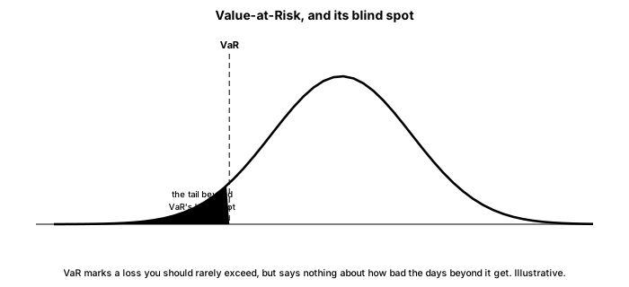
Value-at-Risk, or VaR, is the standard portfolio risk number, and it comes with a famous trap.

# Value-at-Risk (VaR): the loss a portfolio should not exceed on a given day, at a
# given confidence. It is the standard portfolio risk number, and it has a famous
# blind spot. We compute it two ways on fat-tailed daily returns and compare it to
# the worst day that actually happened.
import numpy as np
from scipy import stats

# One year of daily portfolio returns, fat-tailed (Student-t), about 1% typical move.
daily = stats.t.rvs(df=4, size=252, random_state=30) * 0.01
confidence = 0.95

historical_var = -np.percentile(daily, (1 - confidence) * 100)          # from real returns
parametric_var = -(daily.mean() + stats.norm.ppf(1 - confidence) * daily.std(ddof=1))  # normal
worst_day = -daily.min()

print(f"95% one-day Value-at-Risk:")
print(f"  historical (from the returns):  {historical_var * 100:.2f}%")
print(f"  parametric (normal assumption): {parametric_var * 100:.2f}%")
print(f"Worst day that actually happened: {worst_day * 100:.2f}%")

print("\nVaR says: on 95% of days you lose no more than this. It says NOTHING about")
print("how bad the other 5% of days get, and the normal version underestimates the")
print("fat tails from Part 2. The worst day dwarfs the VaR. Manage the tail itself,")
print("and never mistake a single risk number for safety.")

95% one-day Value-at-Risk:
  historical (from the returns):  2.06%
  parametric (normal assumption): 2.21%
Worst day that actually happened: 6.32%

VaR says: on 95% of days you lose no more than this. It says NOTHING about
how bad the other 5% of days get, and the normal version underestimates the
fat tails from Part 2. The worst day dwarfs the VaR. Manage the tail itself,
and never mistake a single risk number for safety.

VaR is the loss your portfolio should not exceed on a given day, at a given confidence. At 95% confidence here, the historical VaR, read from the actual returns, is 2.06%, and the parametric VaR, which assumes a normal distribution, is 2.21%. So on 95% of days you lose no more than about 2%. Now the blind spot. VaR says nothing whatever about how bad the other 5% of days get, and the worst day that actually happened was 6.32%, three times the VaR. Worse, the parametric version is built on the normal distribution, which the fat tails from Part 2 make a serious underestimate of extreme days. VaR is a useful summary and a dangerous single number: an over-reliance on it helped large banks convince themselves they were safe before the 2008 crisis. Manage the losses beyond VaR, sometimes measured by the expected shortfall (the average loss on the worst days), and never mistake a comforting VaR figure for safety.

Factor exposures and neutralisation

Beyond how much risk you carry, a quant watches which risks. A portfolio you believe is a pure value bet might secretly carry a large bet on small caps, or on the market as a whole, exposures you did not choose and are not being paid to take. Measuring your exposure to each factor, and to the market, is core quant risk management, and neutralising the unwanted ones is a common move. Hedging out the market exposure, for instance, turns a strategy market-neutral, so it profits from the factor whether the market rises or falls. The goal is to be paid for the risks you deliberately took and not to be blindsided by ones you did not know were there.

Stress testing and the off-switch

Two final tools. Stress testing asks how the book would fare in events the normal model cannot imagine: a repeat of 2008, a rate shock, a liquidity freeze. Because the tails are fat, you stress beyond what the statistics predict, and size so you survive the stress, not just the average day. And the last tool is the off-switch. An edge that has stopped working, which the next chapter shows is the normal fate of edges, or a risk that has grown past your limit, is a reason to cut size or stop entirely, mechanically and without hope, exactly the kill switch from Algorithmic Trading raised to the level of the whole portfolio. Knowing when to turn a strategy off is as much a part of risk management as knowing how to size it.

What to carry forward

Quant risk management works at the portfolio level. Value-at-Risk measures the loss you should not exceed at a confidence, but its blind spot is the tail it ignores, and its normal version underestimates the fat tails from Part 2, so the worst day here dwarfed the VaR; manage the tail with measures like expected shortfall, not a single comforting number. Control which risks you carry by measuring and neutralising unwanted factor exposures, stress test beyond the normal model, and keep a mechanical off-switch for a strategy that breaks or breaches a limit. You can now find, test, combine, size, and risk-manage edges. The final part faces the honest reality of how rarely all of this pays, and where it sensibly leads.