Trading the spread between two stocks

Every factor so far has been cross-sectional, ranking many stocks at one moment. There is a different family of quant strategies that works in the time dimension: statistical arbitrage, which bets that a stretched relationship between prices will snap back to normal. Its cleanest example is the pairs trade, and it introduces the ideas of mean reversion and cointegration, along with an honest warning that this space is crowded and treacherous.

Mean reversion, and the spread

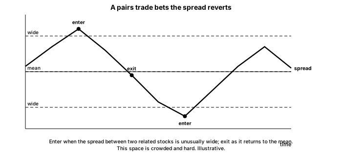
Mean reversion is the tendency of a series to return to its average after straying from it. A single stock's price is mostly not mean-reverting; it is closer to a random walk, wandering with no memory of where it started, which is why chasing a stock because it "must bounce back" is so dangerous. But the spread between two closely related stocks often does mean-revert. If two similar companies normally move together, then when their prices diverge, they tend to converge again, and that convergence is the trade.

Cointegration, in plain terms

The precise idea is cointegration. Two prices are cointegrated if, although each one wanders unpredictably on its own, a particular combination of them, their spread, stays stationary: it hovers around a stable average and keeps returning to it. Stationary simply means the series has a steady mean and spread over time rather than wandering off. A stationary spread is the tradable thing, because you can bet on it returning to its mean with some confidence. The whole craft of pairs trading is finding two stocks whose spread is genuinely stationary and staying alert for when it stops being so.

Building a pairs trade

Here is the trade on a synthetic pair whose spread mean-reverts.

# PAIRS TRADING, the classic statistical arbitrage. Two related stocks tend to
# move together, so the SPREAD between them mean-reverts: when it stretches wide,
# bet it narrows. We build two co-moving price series, form the spread, and trade
# its z-score. Synthetic and illustrative; statsmodels is not required.
import numpy as np

rng = np.random.default_rng(11)
n = 500

# A shared trend both stocks follow, plus a mean-reverting spread between them.
common = np.cumsum(rng.normal(0, 0.01, n))
spread_state = np.zeros(n)
for t in range(1, n):
    spread_state[t] = 0.90 * spread_state[t - 1] + rng.normal(0, 0.02)   # AR(1), reverts
price_a = np.exp(4.0 + common + spread_state / 2)
price_b = np.exp(4.0 + common - spread_state / 2)

# The tradable spread: log A minus log B, standardised into a z-score.
s = np.log(price_a) - np.log(price_b)
z = (s - s.mean()) / s.std()

# Rule: when z is above +1 the spread is stretched wide, so bet it narrows (short
# the spread); when below -1, bet it widens back (long the spread); exit near the
# mean. Act on yesterday's z, so there is no lookahead.
position = np.zeros(n)
for t in range(1, n):
    if position[t - 1] == 0:
        if z[t - 1] > 1.0:
            position[t] = -1
        elif z[t - 1] < -1.0:
            position[t] = 1
    elif abs(z[t - 1]) < 0.5:
        position[t] = 0                          # back near the mean: close
    else:
        position[t] = position[t - 1]

spread_change = np.diff(s, prepend=s[0])
strategy_return = position * spread_change
sharpe = (strategy_return.mean() / strategy_return.std() * np.sqrt(252)
          if strategy_return.std() > 0 else 0.0)
trades = int(np.sum(np.abs(np.diff(position)) > 0))

print(f"Pairs trade on the spread (mean-reversion), {n} days:")
print(f"  round trips (entries and exits): {trades}")
print(f"  annualised Sharpe of the spread strategy: {sharpe:.2f}")
print("\nThe spread mean-reverts, so betting against its extremes pays in this")
print("synthetic pair. In real markets the relationship can BREAK: the two stocks")
print("stop moving together and the spread never comes back. That break is how")
print("pairs trades lose, and testing that the relationship is stable is the hard part.")

Pairs trade on the spread (mean-reversion), 500 days:
  round trips (entries and exits): 45
  annualised Sharpe of the spread strategy: 2.62

The spread mean-reverts, so betting against its extremes pays in this
synthetic pair. In real markets the relationship can BREAK: the two stocks
stop moving together and the spread never comes back. That break is how
pairs trades lose, and testing that the relationship is stable is the hard part.

The strategy forms the spread as the difference in log prices, standardises it into a z-score (how many standard deviations from its mean it sits), and bets against the extremes: when the z-score climbs above one, the spread is stretched wide, so you bet it narrows; when it falls below minus one, you bet it widens back; and you close near the mean. Acting on the previous day's z-score keeps it honest. On this synthetic pair the spread reverts reliably, so the strategy looks excellent. Hold that result at arm's length, because the reality is much harder.

Why it is hard

The flattering result hides every real difficulty. The Sharpe here is high because the data is synthetic with a guaranteed mean-reverting spread, because no trading costs are charged, and because the relationship never breaks. In real markets, all three assumptions fail. Statistical arbitrage is crowded: so many firms run it that the easy spreads are arbitraged thin, leaving tiny margins that costs eat. It is capacity-limited and trades often, so costs and slippage bite hard. And the deadliest risk is that the relationship simply breaks: two companies that tracked each other for years diverge permanently because one is acquired, changes business, or fails, and the spread you bet would revert never comes back, turning a supposedly safe convergence into an open-ended loss. Testing that the cointegration is stable, and cutting a broken pair fast, is the entire difficulty, and it is why statistical arbitrage is far harder than a clean backtest makes it look.

What to carry forward

Statistical arbitrage bets that a stretched relationship reverts, and its classic form is the pairs trade: single stocks wander like random walks, but the spread between two cointegrated stocks stays stationary and mean-reverts, so you standardise it into a z-score and bet against its extremes. The synthetic result looks superb and is deeply misleading, because real pairs trading is crowded, thin, cost-heavy, and above all exposed to the relationship breaking, which turns a sure reversion into an open-ended loss. You have now seen the main families of edge. The next part is the scientific heart of the course: testing any of them honestly enough to know whether it is real.