Many small edges beat one big bet

You have spent Parts 3 and 4 learning how hard it is to find even one real edge, and how weak the real ones are. Here is the good news, and the quant's genuine advantage: you do not need one strong edge. Several weak, independent edges combined can be steadier and better than any one of them, because their good and bad patches partly cancel. This is diversification, applied not to stocks but to strategies, and it is the closest thing to a free lunch in all of finance.

The strength of low correlation

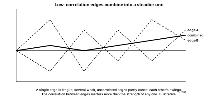
Watch four factors combine into something better than their average.

# Many small edges beat one big bet. We build four factor return series, look at
# how lowly correlated they are, and show that an equal blend beats the average
# factor (and often the best single one), because the factors work at different
# times. Synthetic data (factor_data.py).
import numpy as np
import pandas as pd
from factor_data import make_market, long_short, annual_sharpe

returns, static = make_market()
T = len(returns)


def broadcast(col):
    return pd.DataFrame([static[col].values] * T, columns=returns.columns, index=returns.index)


factors = pd.DataFrame({
    "value":    long_short(broadcast("earnings_yield"), returns),
    "quality":  long_short(broadcast("roe"), returns),
    "momentum": long_short((1 + returns).rolling(12).apply(np.prod, raw=True).shift(1) - 1, returns),
    "lowvol":   long_short(-returns.rolling(12).std().shift(1), returns),
}).dropna()

print("Individual factor Sharpes:")
for name in factors.columns:
    print(f"  {name:9s} {annual_sharpe(factors[name]):.2f}")
avg_individual = np.mean([annual_sharpe(factors[c]) for c in factors.columns])

print("\nCorrelation matrix (low correlation means good diversification):")
print(factors.corr().round(2).to_string())

blend = factors.mean(axis=1)                 # equal-weight blend of the four factors
print(f"\nAverage individual factor Sharpe: {avg_individual:.2f}")
print(f"Equal-blend Sharpe:               {annual_sharpe(blend):.2f}")
print("\nThe blend beats the average factor because the factors are lowly correlated.")
print("Diversification of edges, not the strength of any one, is the quant's most")
print("durable advantage: several weak, uncorrelated edges are steadier than one strong bet.")

Individual factor Sharpes:
  value     1.27
  quality   0.75
  momentum  0.98
  lowvol    0.59

Correlation matrix (low correlation means good diversification):
          value  quality  momentum  lowvol
value      1.00    -0.11      0.22   -0.02
quality   -0.11     1.00     -0.03   -0.11
momentum   0.22    -0.03      1.00    0.21
lowvol    -0.02    -0.11      0.21    1.00

Average individual factor Sharpe: 0.90
Equal-blend Sharpe:               1.68

The blend beats the average factor because the factors are lowly correlated.
Diversification of edges, not the strength of any one, is the quant's most
durable advantage: several weak, uncorrelated edges are steadier than one strong bet.

The four factors have individual Sharpes ranging from 0.59 to 1.27, averaging 0.90. Look at their correlations: mostly near zero, some slightly negative, meaning they tend to work at different times. Now the equal blend has a Sharpe of 1.68, higher than the average factor and higher even than the best single one, value at 1.27. That lift is pure diversification. Because the factors rise and fall out of step, the blend's swings are much smaller than any single factor's, while its return is the average of theirs, and a smaller denominator with the same numerator is a higher Sharpe. The lower the correlations, the larger the benefit.

Correlation matters more than strength

Here is the insight that reorders your priorities. When you are combining edges, the correlation between them matters more than the strength of any one. Two mediocre edges that are uncorrelated can beat one strong edge alone on a risk-adjusted basis, because the pair diversifies and the loner does not. This flips the beginner's instinct. Do not hunt for the single perfect strategy; collect several decent, genuinely different ones, and let their independence do the work. It also tells you what to protect. The whole benefit rests on the edges staying uncorrelated, and correlations have a cruel habit of rising toward one in a crisis, when everything falls together and the diversification you counted on vanishes exactly when you needed it. So a quant watches not just each edge but how they move together, especially in bad times.

What to carry forward

The quant's durable advantage is not one strong edge but several weak, uncorrelated ones combined, because their ups and downs partly cancel and the blend is steadier than any part, lifting the Sharpe above the average factor and even the best single one. For combining, correlation matters more than strength: collect several different decent edges rather than hunting one perfect one. And guard the correlations, because they rise toward one in a crisis, when you need the diversification most. Holding several edges together raises the next question: how much of each to hold, which is portfolio construction.