Backtesting a whole portfolio

The backtest you built in Python for Trading traded a single asset in and out. A quant backtest is a different animal: a whole portfolio of many stocks, rebalanced on a schedule, where each period you re-rank the universe and adjust your holdings. This chapter builds that portfolio backtest, and adds the cost of trading that a serious test can never leave out.

From one asset to a portfolio

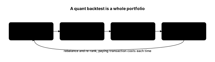
A portfolio backtest runs a simple cycle. Each period, monthly here, you rank the universe by your factor, select the stocks to hold, usually a top slice like the best 20%, weight them, and hold to the next rebalance. Equal weighting, giving each held stock the same share, is the honest default, because fancier weighting is easy to overfit. The portfolio's return for the period is the weighted average of its holdings' returns, and stringing these together across the whole history gives the strategy's return series. This is a long-only portfolio; a long-short strategy runs the same cycle for a short book too, as the factor chapters did.

Rebalancing and the cost of turnover

Because a dynamic factor re-ranks the market each period, the holdings change, and changing holdings costs money. Here is the full cycle with that cost included.

# A quant backtest is not one asset traded in and out, but a whole PORTFOLIO
# rebalanced on a schedule. Here we build a long-only momentum portfolio: each
# month, hold the top 20% of stocks by trailing return, equally weighted, rebalance,
# and charge a cost on the fraction of the book that turns over. Synthetic data.
import numpy as np
import pandas as pd
from factor_data import make_market, annual_sharpe, max_drawdown

returns, static = make_market()
n_months, n_stocks = returns.shape
k = max(1, int(n_stocks * 0.2))
cost_rate = 0.002               # 0.2% cost on the fraction of the book traded

momentum = (1 + returns).rolling(12).apply(np.prod, raw=True).shift(1) - 1

prev_weights = pd.Series(0.0, index=returns.columns)
gross_list, net_list, turnover_list = [], [], []
for t in returns.index:
    scores = momentum.loc[t].dropna()
    if len(scores) < k:
        continue
    winners = scores.sort_values(ascending=False).index[:k]
    weights = pd.Series(0.0, index=returns.columns)
    weights[winners] = 1.0 / k                          # equal-weight top quintile
    turnover = (weights - prev_weights).abs().sum() / 2  # fraction of book traded
    gross = (weights * returns.loc[t]).sum()
    gross_list.append(gross)
    net_list.append(gross - turnover * cost_rate)
    turnover_list.append(turnover)
    prev_weights = weights

gross = pd.Series(gross_list)
net = pd.Series(net_list)
print(f"Long-only momentum portfolio (top 20%, monthly rebalance), {len(net)} months")
print(f"  gross cumulative return: {((1 + gross).prod() - 1) * 100:6.1f}%")
print(f"  net cumulative return:   {((1 + net).prod() - 1) * 100:6.1f}%   (after costs)")
print(f"  average monthly turnover:{np.mean(turnover_list) * 100:5.0f}% of the book")
print(f"  net annualised Sharpe:   {annual_sharpe(net):6.2f}")
print(f"  net maximum drawdown:    {max_drawdown(net) * 100:6.1f}%")
print("\nA quant backtest is a whole portfolio, rebalanced on a schedule, with costs")
print("charged on the turnover, which is why a high-turnover factor loses more to costs.")

Long-only momentum portfolio (top 20%, monthly rebalance), 60 months
  gross cumulative return:   98.2%
  net cumulative return:     93.1%   (after costs)
  average monthly turnover:   22% of the book
  net annualised Sharpe:     1.02
  net maximum drawdown:     -16.2%

A quant backtest is a whole portfolio, rebalanced on a schedule, with costs
charged on the turnover, which is why a high-turnover factor loses more to costs.

Each month the momentum ranking shifts, so the portfolio sells some names and buys others. The fraction of the book that changes is the turnover, about 22% a month here, and a cost is charged on it. The effect is visible: a gross cumulative return of 98.2% became 93.1% after costs over five years, a drag of around five percentage points, and a higher-turnover factor would lose more. The net Sharpe is 1.02 with a maximum drawdown of 16.2%. Those three additions, many holdings, periodic rebalancing, and turnover-based costs, are what make a quant backtest a portfolio test rather than a single-asset one.

The honest-backtest discipline carries over

Everything Python for Trading insisted on applies here at larger scale: act only on information available at the time, charge realistic costs, and never let the future leak in. On top of that sit the data disciplines from Part 2: adjusted prices, point-in-time fundamentals, and a survivorship-free universe. A portfolio backtest with any of those wrong is exactly as false as a single-asset one that cheats, only bigger and more convincing. The machinery is more elaborate, but the rule is unchanged: a backtest is a hypothesis to doubt, not a promise.

What to carry forward

A quant backtest runs a portfolio cycle: each period rank the universe, hold a top slice equally weighted, rebalance, and compound the returns, charging a cost on the turnover, which you saw drag a 98.2% gross return down to 93.1% net at 22% monthly turnover. The honest-backtest rules from Python for Trading and the data rules from Part 2 apply at this larger scale, and a portfolio test that breaks them is just a bigger lie. With a portfolio return series in hand, the next question is how to judge it, and the answer is never the return alone.