Less risk, more return

The most surprising factor in finance says that the calmest stocks have delivered strong risk-adjusted returns, which flatly contradicts the textbook idea that more risk must mean more return. That is the low-volatility anomaly, and alongside the older, weaker size factor, it rounds out the defensive core of a factor portfolio.

Low volatility, and the surprise

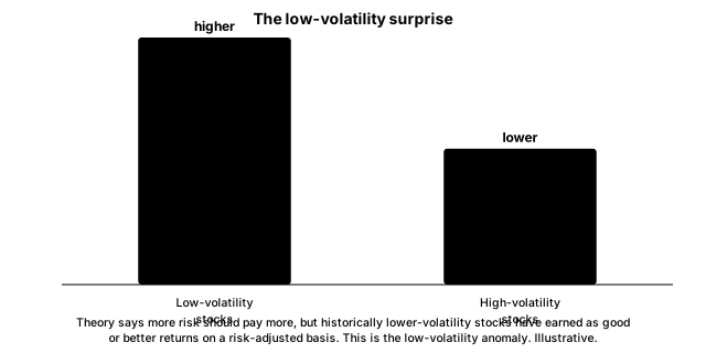
The low-volatility factor buys the calmest stocks, those with the smallest ups and downs, and avoids or shorts the wildest.

# LOW VOLATILITY and SIZE. The low-volatility factor buys the calmest stocks, and
# its historical strength is one of finance's surprises, because naive theory says
# more risk should mean more return. The size factor buys smaller companies. We
# build both as long-short factors. Synthetic, illustrative data (factor_data.py).
import numpy as np
import pandas as pd
from factor_data import make_market, long_short, annual_sharpe, max_drawdown

returns, static = make_market()
n_months = len(returns)

# Low volatility: rank by trailing 12-month return volatility (calmer = higher
# score), shifted so month t uses only past returns.
low_vol_score = -returns.rolling(12).std().shift(1)
low_vol = long_short(low_vol_score, returns, quantile=0.2)

# Size: rank by market capitalisation, smaller = higher score.
size_score = pd.DataFrame([-np.log(static["market_cap"].values)] * n_months,
                          columns=returns.columns, index=returns.index)
size = long_short(size_score, returns, quantile=0.2)

print(f"Low-volatility factor  Sharpe: {annual_sharpe(low_vol):5.2f}  "
      f"maxDD: {max_drawdown(low_vol) * 100:.1f}%")
print(f"Size factor            Sharpe: {annual_sharpe(size):5.2f}  "
      f"maxDD: {max_drawdown(size) * 100:.1f}%")
print("\nLow volatility has historically delivered solid risk-adjusted returns,")
print("which naive theory does not predict, making it a favourite defensive factor.")
print("Size is a weaker, less reliable factor, as its low Sharpe here reflects.")

Low-volatility factor  Sharpe:  0.59  maxDD: -28.3%
Size factor            Sharpe:  0.30  maxDD: -16.4%

Low volatility has historically delivered solid risk-adjusted returns,
which naive theory does not predict, making it a favourite defensive factor.
Size is a weaker, less reliable factor, as its low Sharpe here reflects.

The strategy ranks stocks by their trailing return volatility and favours the quiet ones, earning a Sharpe of about 0.6 in this illustrative data. Why is this surprising? Because the standard theory, the one behind the capital asset pricing model, says higher risk should be rewarded with higher return, so the wildest stocks should win. Empirically, across decades and markets, they have not: calm stocks have matched or beaten volatile ones on a risk-adjusted basis. The leading explanation is behavioural. Investors overpay for exciting, lottery-like volatile stocks, hoping for a jackpot, which leaves them expensive and the boring calm stocks underpriced. It is the NSE's low-volatility index and a favourite defensive factor. Note, though, the higher drawdown even here: defensive does not mean safe, only steadier on average.

Size, the weak old factor

The size factor says smaller companies have historically outperformed larger ones, the small-cap premium. It is one of the oldest documented effects, and also one of the least reliable. Its illustrative Sharpe here, about 0.3, is the weakest of all our factors, and in reality the size premium has largely faded in developed markets and is unstable. Small caps also carry exactly the traps the data chapters warned about: thin liquidity that makes fills costly, and a survivorship bias that flatters backtests because so many small companies fail. Treat size as a weak, cautious factor, useful mainly in combination and never leaned on alone.

The defensive core

Put the defensive factors together and a picture emerges. Low volatility and quality, from the last chapter, are the steady, defensive tilts: they tend to lose less when markets fall and to avoid the violent crashes that momentum suffers. A sensible factor portfolio often centres on these defensive factors and adds the more aggressive value and momentum around them, rather than the other way around. The calmest core is usually the wisest core, a theme the portfolio-construction chapters develop.

What to carry forward

The low-volatility factor buys the calmest stocks and has delivered strong risk-adjusted returns, contradicting the theory that risk must be rewarded, likely because investors overpay for volatile lottery stocks. With quality, it forms the defensive core a sensible factor portfolio is built around. The size factor is old but weak and unreliable, and small caps carry the liquidity and survivorship traps from Part 2, so it deserves only a light touch. You have now met the main cross-sectional factors. The last chapter of this part steps into a different family entirely, betting on relationships rather than rankings: mean reversion and pairs trading.